In this final section on time series analysis, we’ll look in more detail at two of the models (ARIMA and SARIMA) that are available to you to explore time-series data in R.
This will build on previous material, and introduce some additional concepts and techniques you may find useful.
60.2 ARIMA Models
ARIMA models (AutoRegressive Integrated Moving Average models) are commonly-used tools in time-series analysis, especially for forecasting future trends based on past data.
Like the other models covered previously, they help us predict future values in a sequence of data by analysing past values.
The “AR” part stands for AutoRegressive. This means the model looks at previous data points and uses these to predict future ones. It’s like trying to guess the next number in a sequence by looking at the numbers before it.
The “I” in ARIMA stands for Integrated. ARIMA models make the time-series data more consistent and stable over time, often by removing trends or seasonal effects.
Lastly, the “MA” part stands for Moving Average. ARIMA models smooth out short-term fluctuations in the data, and highlight longer-term trends or cycles.
60.3 SARIMA (Seasonal ARIMA) Models
SARIMA models are really an extension of the ARIMA model. They are designed to better handle seasonal variations in time-series data which, as we’ve previously covered, can mask the ‘real’ trends and patterns within time-series data.
SARMIA models are structured to include both non-seasonal and seasonal elements. The full notation for a SARIMA model is SARIMA(p, d, q)(P, D, Q)m.
Here’s what each of these components represents:
Non-Seasonal Components:
p (AutoRegressive Order): the number of lagged observations in the model. For instance, p = 2 would use the first two lagged values (like using data from the previous two months to predict this month’s value).
d (Integrated Order): the number of times the data needs to be differenced to make it stationary, meaning to stabilise the mean over time. For instance, if the data shows a linear trend, you might need to difference it once (d = 1) to remove that trend.
q (Moving Average Order): the size of the moving average window. It uses the error terms from the past forecasted values to improve the model’s accuracy.
Seasonal Components:
P (Seasonal AutoRegressive Order): similar to ‘p’, but for the seasonal part of the model. It represents the number of seasonal lags of the dependent variable that the model will use.
D (Seasonal Integrated Order): the number of seasonal differences required to make the series stationary.
Q (Seasonal Moving Average Order): similar to ‘q’, but for the seasonal part of the model. It represents the order of the moving average for the seasonal differences.
m (Seasonality Period): the number of time steps for a single seasonal period. For example, m = 12 for monthly data with an annual cycle.
Again, the strength of SARIMA models is their ability to decompose a time-series into seasonal and non-seasonal components and analyse these elements separately yet simultaneously. This usually provides a more accurate forecast in seasonally-affected time series data than we get from ARIMA.
60.4 An example of ARIMA and SARIMA on the same dataset
In this example, I’m going to use a dataset with a strong seasonal element.
# Load necessary librarieslibrary(forecast)
Registered S3 method overwritten by 'quantmod':
  method            from
  as.zoo.data.frame zoo
set.seed(123) # For reproducibilityseasonal_component <-sin(seq(1, 120, length.out =120) *2* pi /12) *10time_series_data <-ts(rnorm(120, mean =10, sd =5) + seasonal_component, frequency =12)
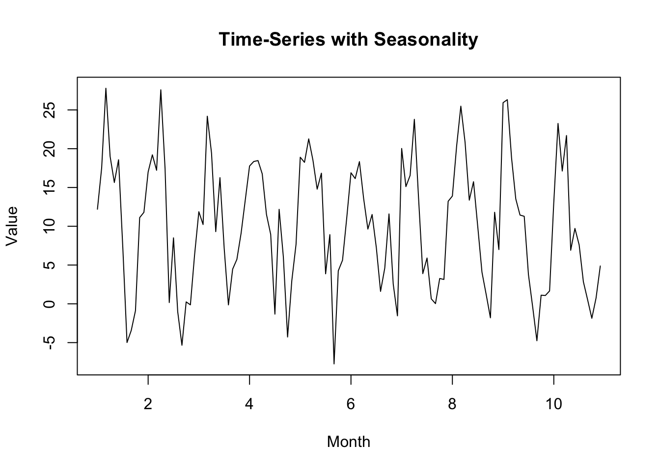
I’ll plot the dataset to facilitate an initial exploration.
# Plot datasetplot(time_series_data, main ="Time-Series with Seasonality", xlab ="Month", ylab ="Value")
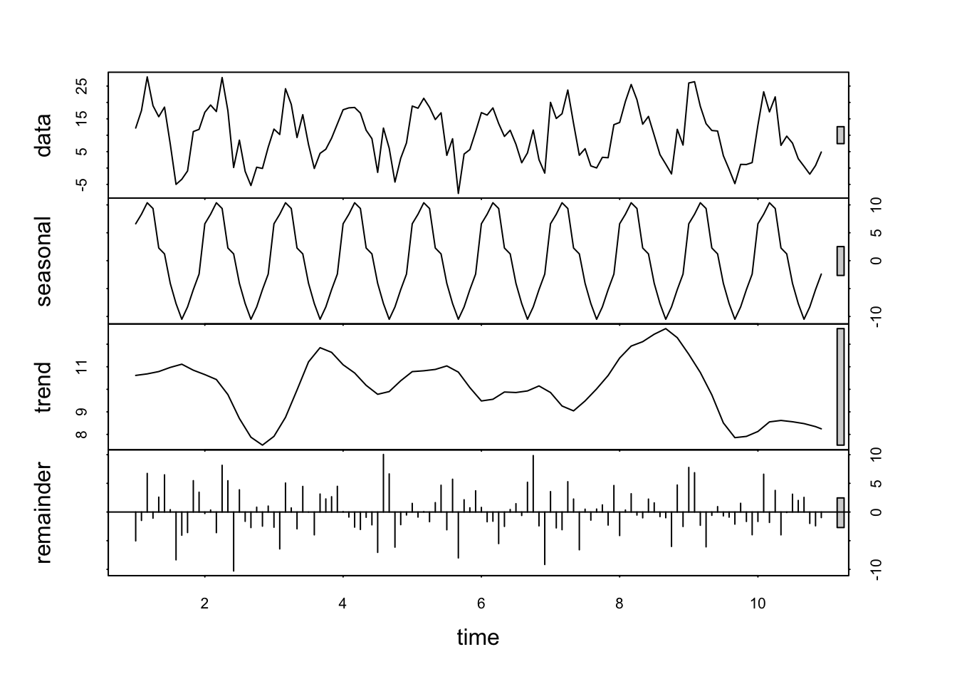
If I break this time-series down (decompose) into its constituent parts, the seasonality in the data should become clear:
We can see a very clear seasonal pattern in the data. If we don’t take this into account, we’re going to have problems when we try to create predictive models using this data.
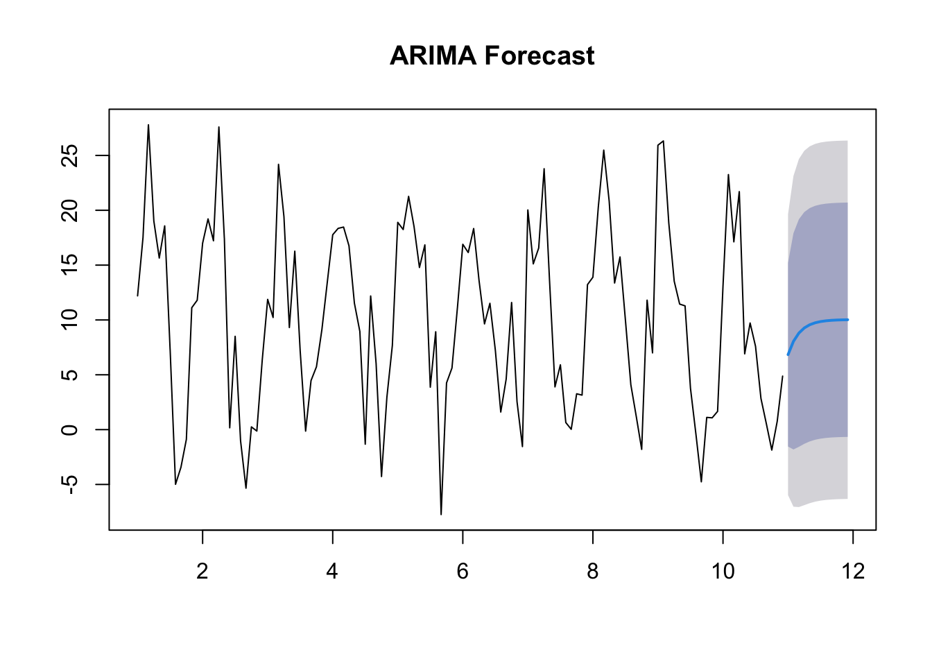
In the first attempt to build a predictive model from this data, I’ll run an ARIMA model. Remember that this is not the optimum approach, because I know there may be seasonality within my data. However, I’ll run it anyway to demonstrate the difference between ARIMA and SARIMA:
Series: time_series_data
ARIMA(1,0,0) with non-zero mean

Coefficients:
         ar1     mean
      0.6204  10.0366
s.e.  0.0707   1.5384

sigma^2 = 42.74:  log likelihood = -394.82
AIC=795.64   AICc=795.85   BIC=804.01

Training set error measures:
                      ME     RMSE      MAE       MPE    MAPE     MASE
Training set -0.01512718 6.483211 5.120995 -99.28832 389.089 0.916242
                   ACF1
Training set 0.04754608
forecast_arima <-forecast(arima_model, h =12)plot(forecast_arima, main ="ARIMA Forecast")
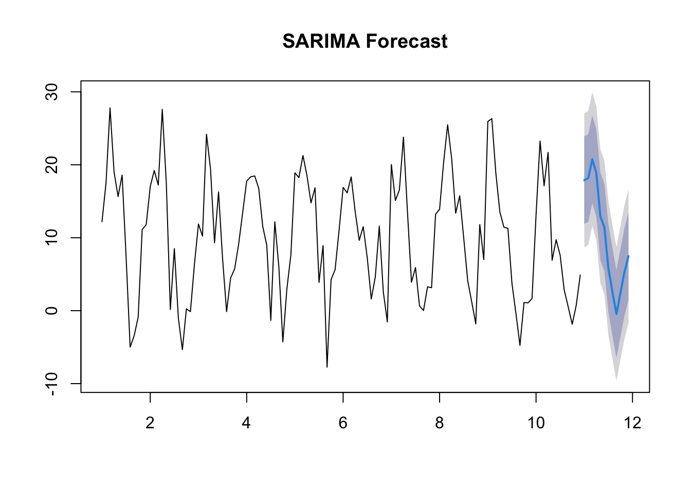
I’ll also run a SARIMA model on the same time-series:
Series: time_series_data
ARIMA(0,0,0)(0,1,2)[12]

Coefficients:
         sma1    sma2
      -1.0450  0.1803
s.e.   0.1533  0.1146

sigma^2 = 21.71:  log likelihood = -327.85
AIC=661.7   AICc=661.94   BIC=669.75

Training set error measures:
                     ME     RMSE     MAE      MPE    MAPE      MASE       ACF1
Training set -0.2040055 4.379059 3.28606 3.637575 226.066 0.5879376 0.04117254
forecast_sarima <-forecast(sarima_model, h =12)plot(forecast_sarima, main ="SARIMA Forecast")
You can see that, even from a visual perspective, the output of ARIMA (which ignores the seasonal element) appears much less useful in terms of future forecasting than SARIMA, which takes the seasonal element into account.
We can confirm this by looking at the AIC for the SARIMA model which, at 661.7, is lower than that for the ARIMA model (795.6), indicating the the SARIMA model is more effective (or a better ‘fit’ to the data).